4 Applications

4.1 Causality and Machine Learning

Machine learning has seen many successful applications in recent years. Methods most often employed today belong to the unsupervised and supervised learning paradigm. These methods assume that observed data are identically and independently distributed samples of a (super-) population. For example, supervised learning techniques attempt to learn $Y$ from a set of variables $X$, i.e. trying to learn $P(Y|X) = f(X)$. From the discussion so far it should become clear that only few problems are fit for this paradigm. If $X$ and $Y$ are produced by the same causal/physical system, it should be able to learn the form of $f()$ by collecting lots of data points and fitting algorithms that function class. For example, the “hello world” example of machine learning consists of recognizing handwrittern letters. It is reasonable to assume that this is a rather stable relationship. There aren’t so many different ways people write letters once you’ve seen houndreds of thousands of them. It is also likely that there is no evolution of that relationship, that observervations taken a year ago are not that different from those taken now. It should also be likely that you can transfer this relationship reasonably well between physical systems that do the same or a similar thing, e.g. handwritten letters from tablets vs phones. Transfer will not as well work if the physical system is quite different, e.g. writing with a pen on paper rathen than with a stylus on a digital device.

Many important systems, however, are constantly evolving. It is not reasonable to assume that movie recommendations will be stable over time. Recommending a new show that is currently all the buzz, might not be a good recommendation in a year. Customers who haven’t chosen to see this show yet, might be well aware of the show, but have deliberately decided not to watch it. Using the same trained recommendation model over a prolonged time-period might lead to ever-decreasing model performance and will hence require constant re-training. Models then do not always get better and better over time as information from past observations depreciates in value quite quickly.

Some systems are evolving much quicker than data becomes available. The (world) economy is such a system. Individual behavior and choices are continuously refined and can dramatically change on short notice, while most (macro-) economic data might only be available on a weekly or monthly basis. Innovation plays an important role. The action set is not fixed over time, but evolves constantly. It can neither be modelled nor predicted (it wouldn’t be an invention then)

4.2 Marketing

Another common application where correlation is often confused with causation is in marketing. This might be because data scientist and business might not speak the same language. It might, however, also be a valid pragmatic assumption, which is later validated in an experiment. I will focus here on the (mis-)application of propensity modeling. Propensity modeling attempts to predict if a (potential) customers will perform a certain action, e.g. whether a new visitor on your site will register or whether a customer will buy a certain product. The model output is an estimated probability that the customer will do the action. Propensity models therefore fall into the class of binary regression.

\[\begin{equation} P(Y|I) = f(I) \label{eq:mktg1} \tag{1} \end{equation}\] where $I$ is the information set available for prediction.⁵

There are plently of algorithms that could be used to estimate the function. Logistic regression is often chosen as it is easy to implement and the model itself might provide some insights. Here, we will focus not on the implementation part, but on the interpretation and (mis-) use of the model.

To see why the model might not be want you think it is, we will have a A naive usage of the model is to focus marketing on customers with high likelhood to do the action. This however, can be serverly misleading, as we will discuss next. To show this, we will start with an ideal assumption: our model is perfect. A perfect model means that we predict the customer action correctly for every customer and the model produces predicted probabilies which are well calibrated. This means that we only get two predictions, either a customer will do action with estimated probability 0 or whether they will do so with probability 1 - and the model is always right. However, although we have the best possible model, it illustrates well why the naive interpreation cannot be correct. If we focus our marketing on those customers with highest propensity (as there are only two values it is those with predicted probability 1), we focus our attention on a customer group that buys the product anyways. In fact, these are the customers that we should least focus on as the best we can do is to have no effect on those customers (but we still have the cost of the marketing intervention, which might be an opportunity cost) and in some case we might even affect the customer adversely (as they might be annoyed by the marketing). Hence, we’re left with the second group of customers, those with predicted probability of 0. In this group, there might be some who will be convinced to buy the product after being exposed to the marketing, but we are not able to say which ones. Even after doing an experiment, we will not improve on our decision rule. Say, we run an A/B test on all customers who were predicted to not buy, and we estimate that 0.02 Depending on the situation, this model might not be very useful. The only thing that we learned from the model is that we should exclude those customers with highest probability from our marketing. This runs counter to our intuition. Furthermore, in many applications, the action might be a rare event, with likelihoods not much higher than 1%. Excluding these customers from marketing might not save a lot of money in the first place, and establishing a system where you’re able to provide different marketing on customer-level might have some fixed costs (e.g. it might require to store and process customer-level data and deploy the model-outputs to production systems).

From the example it becomes clear that propensity modelling using a predictive model on passively observed data will at best be a proxy for the problem at hand. The goal of marketing optimization is to optimally trade-off the cost and effect of marketing, where the latter is a causal rather than an assosiative concept. Supervised machine learning models, regardless of their complexity, will fail at achieving the task since even a ideal falls short. To see this more clearly, let’s restate the problem in causal notation first. Let $Y$ denote the binary customer action we want to predict. Further, let $S$ denote the default environment, which includes all relevant causal factors that determine customer decisions, their preferences and endowment, the offers available on the market and our own offer and current marketing strategy. For simplicity’s sake, let’s assume our marketing strategy is binary and denote it by $M$ (e.g. whether or not we send the customer a marketing email). Assume the current marketing strategy is $M = 0$, i.e. we do currently not have an email program. The individual causal differential effect of sending an email to customer $i$ is then \[\begin{equation} \Delta_i := Y_i^{S;do(Z_i:=1)} - Y_i^{S; do(Z_i:=0)} \label{eq:myfirsteq} \tag{1} \end{equation}\]

As $Y$ is binary, $\Delta$ can be one of ${-1, 0, 1}$ with $\Delta = 1$ being the desired outcome. As discussed in [causality], we are not able to measure this quantity directly, but need to resort to population-level quantities instead: \[\begin{equation} P(\Delta) = P^{S;do(Z:=1)}(Y) - P^{S;do(Z:=0)}(Y) \label{eq:mktg_pop_ate} \tag{2} \end{equation}\] Both quantities on the right-hand side of equation $\eqref{eq:mktg_pop_ate}$ can be estimated. There are couple of ways to do so, many of which we discussed in [causality]. The most straigtforward way is to apply a randomized controlled trial (or “A/B test”) where the population at hand is randomly split in two groups, one group being exposed to the marketing (i.e. $S;do(Z:=1)$) the other not being exposed (i.e. $S;do(Z:=0)$). Conditioning the probability estimate on a set of features allows us to investigate whether the differential causal effect is co-related with observable information - which ultimately tells us who will be most affected by the marketing. In the most simple case, we condition by a single discrete attribute $A$, providing \[\begin{equation} P(\Delta | A) = P^{S;do(Z:=1)}(Y | A) - P^{S;do(Z:=0)}(Y | A) \label{eq:mktg_pop_cate} \tag{3} \end{equation}\]

This is superficially similar to equation $\eqref{eq:mktg1}$, but note that the right-hand side in $ describes two conditional probabilities drawn from two different environments. It will be helpful to rewrite this into a linear model form. Assume that $A$ is binary. Then \[\begin{align} P(\Delta | A = 1) &= P^{S;do(Z:=1)}(Y | A = 1) - P^{S;do(Z:=0)}(Y | A = 1) \\ &= a_1 - a_0 \\ &=: \Delta_1 \\ P(\Delta | A = 0) &= P^{S;do(Z:=1)}(Y | A = 0) - P^{S;do(Z:=0)}(Y | A = 0) \\ &= a_3 - a_2 \\ &=: \Delta_0 \end{align}\] We can further represent $P(Y)$ as a function of $Z$ \[\begin{align} P(Y) &= P^{S;do(Z:=0)}(Y) \cdot (1-Z) + P^{S;do(Z:=1)}(Y) \cdot Z \\ &= P^{S;do(Z:=0)}(Y) + (P^{S;do(Z:=1)}(Y) - P^{S;do(Z:=0)}(Y)) \cdot Z \\ &= P^{S;do(Z:=0)}(Y) + P(\Delta) \cdot Z \\ &= \beta_0 + \beta_1 Z \end{align}\] Further, replacing unconditional quantities with conditional ones, we can write \[\begin{align} P(Y | A) &= P^{S;do(Z:=0)}(Y | A) + P(\Delta | A) \cdot Z \\ &= \alpha_0 + \alpha_1 A + (\Delta_0 + \Delta_1 \cdot A) \cdot Z \\ &= \alpha_0 + \alpha_1 A + \Delta_0 Z + \Delta_1 A Z \end{align}\] which looks quite familiar as it is the conventional way to specify a logistic regression equation on $A$, $Z$ and the interaction of both $A \cdot Z$.[^footnote-hte-nomenclature] If the treatment is ineffective $\Delta_0 = 0$ and $Delta_1 = 0$. The differential causal effect is said to be heterogeneous, if $\Delta_1 \neq 0$. [^footnote-hte-nomenclature]: The literature on heterogeneous treatment effect models often groups parameters of this equation regarding their role in application: $\alpha_1$ is called “prognostic” as it shows if and how the success rate differs across attributes $A$ if no intervention/treatment is provided; $\Delta_1$ on the other hand is often called “predictive”, meaning how predictive $A$ is on the effectiveness of the intervention/treatment, i.e. whether and by how much treatment effects differ across values of $A$.

The model can be generalized to the case where not just a single (binary) attribute is considered, but a vector of attributes.

In a marketing context with binary treatment and outcome, table xxx can be restated as

Table 4.1: Caption here
	$Y^{\Gamma;do(X:=0)} = 0$	$Y^{\Gamma;do(X:=0)} = 1$
$Y^{\Gamma;do(X:=1)} = 0$	“Lost Cause”	“Do-Not-Disturb”
$Y^{\Gamma;do(X:=1)} = 1$	“Persuadable”	“Sure Things”

4.3 Drug Trial

4.4 Discrimination

In den letzten Jahren wurde in Politik, Medien und Wissenschaft häufiger über Diskriminierung diskutiert, einige Beispiele sind hierbei die Diskriminierung von Frauen im Berufsleben, der Wahl von Abegordneten zum Bundestag. Ein Verbot von Diskriminierung hat in Deutschland im Jahre 2006 Gesetzescharakter angenommen mit der Verabschiedung des Allgemeinen Gleichbehandlungsgesetzes (AGG), dass u.a. die Diskriminierung aus Gründen des Alters, der ethnischen Herkunft oder des Geschlechts unzulässig ist. Wie bereits des Gesetzesname andeutet, wird Diskriminierung als ein Vorgang angesehen, nicht als ein Zustand. Dies wird insebesondere in §3 deutlich, wo eine (unmittelbare) Diskriminierung dann vorliegt “wenn eine Person wegen [Alter, Herkunft oder Geschlecht] eine weniger günstige Behandlung erfährt, als eine andere Person in einer vergleichbaren Situation erfährt”. Die zunehmende Anwendung automatisierter Entscheidungsalgorithmen rückt die Frage nach Diskrimierung auch in den Blickpunkt der Forschung im Bereich des maschinellen Lernens. Es ist in diesem Kontext, dass dieses Thema eine mathematische Formalisierung erfahren hat. Dabei wurden zuletzt auch kausale Argumentationen und Notation eingeführt, siehe etwa Kilbertus etl al..

Wir werden uns im Folgenden an einem einfachen Beispiel diesem Problem nähern sowie einen Versuch der Die Identifikation von diskriminierenden Handlungen wird dadurch erschwert, dass die Handelnden Personen häufig nur einen Teil des gesamten Mechanismus kontrollieren und es begründete Sachzwänge gibt. Im Folgenden unterscheiden wir zwei Merkmalstypen

First, let’s introduce some basic terminology first: * protected feature: this is a person’s feature that is legally protected, e.g. age or gender. * accepted feature: these are features that are explicitely or implicitely accepted for discrimination, e.g. the job might (by law) require a certain certificate of qualification or the job requires a certain skillset like a specific programming language or the ability to lift weigths heavier than 30 kg.

While the protected features are usually unambiguous and explicitly stated in law, the accepted features can be reason for disagreement. It is usually the set of features that are deemed to be necessary to do the job, but of course “doing the job” can done in different qualities. A bar owner might believe it to be necessary for his waiters to be handsome and flirty with the predominantely female audience, but an applicant might think it is not. Getting the order right and providing the right servcie while being friendly he might consider to be sufficient.

unprotected feature: these are all features that are not explicitly protected, e.g. eye color, ability to lift more than 30kg
zulässige Merkmale: dies sind Merkmale, nach denen eine diskriminierende Handlung zulässig ist. So kann etwa für eine Tätigkeit in einem Warenlager voraussgesetzt werden, dass ein Bewerber in der Lage sein muss, Lasten über 20kg zu transportieren, da dies für die Erfüllung der Tätigkeit unabdingbar ist.
aufhebende Merkmale: diese stellen eine Teilmenge der zulässigen Merkmale dar. Es sind diejenigen Merkmale, die auf dem kausalen Pfad zwischen den geschützten Merkmalen und dem Output liegen. Das Merkmal “kann Lasten über 20kg transportieren” ist vermutlich ein solches, da dieses kausal vom Geschlecht und/oder dem Alter eines Bewerbers beeinflusst ist.
unzulässige Merkmale: sind Merkmale, nach denen eine diskriminierende Handlung nicht zulässig ist, die aber nicht ein geschütztes Merkmal sind. Dies könnte etwa die Augenfarbe des Bewerbers sein, die (etwa gemäß AGG nicht geschützt ist), jedoch für die Erfüllung der Tätigkeit irrelevant sein dürfte.
stellvertretende Merkmale: diese stellen eine Teilmenge der unzulässigen Merkmale dar. Es sind diejenige Merkmale, die auf dem kausalen Pfad zwischen den geschützten Merkmalen und dem Output liegen. So kann die Augenfarbe eines Bewerbers ein stellvertretendes Merkmal sein, wenn die Augenfarbe etwa durch das Geschlecht oder die ethnische Herkunft beeinflusst wird. Sie werden stellvertretend genannt, da sie Information über das geschützte Merkmals beinhalten und somit zur Diskriminierung herangezogen werden könnten.

TODO: sollte unzulässig nicht anders bezeichnet werden, da ja eine Diskriminierung nach nicht-stellvertretern rechtlich nicht verboten ist.

Es gelten folgende Definitionen:

kann ein Mechanismus der unmittelbaren Diskriminierung durch einen vom geschützten Merkmal unabhängigen Prozess (oder eine Konstante) ersetzt werden, ohne dass sich die Verteilung der Zielvariable ändert, so ist dieser Mechanismus nicht-diskriminierend

4.5 Epidemiology

Inspired by the SARS-CoV-2 epidemic of 2020, let’s have a look at a causal model for aggregate epidemiological data. During the epidemic, the numbers of infected and deceased have been widely reported in news outlets throughout the world and (especially in the beginning) have been closely monitored by millions on a daily basis. Soon, the reported numbers have raised many questions as they suggested wildly different conclusions about the virus’ lethality across countries. While the WHO reported a case-fatality-rate (CFR) of 3.5%, some countries reported CFRs as low as 0.3%. Differences in pogress of the pandemic, demographics, and the availability of intensive-cars-units (ICU) would suggest some differences, but a deviation by an order of magnitude seemed unlikely

The differences in reported numbers and statistics are understood to be substantially driven by differences in the data generation process, especially the mechanism of who is subjected to a test for the virus. While South Korea adopted a strategy of widespread testing of the population, others only tested when patients showed (severe forms) of associated symptoms and/or recent contact with known infected people.

To illustrate this, we will model parts of the data generating process as causal mechanisms, allowing us to reason about the effects of different testing strategies on reported numbers, how we can estimate the number of patients who died because of the virus rather than died with the virus, and how government measures (lockdown) fit into this model.

In a second part, we swith focus a little bit and take a closer look at the dynamics of the pandemic. We show how dynamic systems can be represented in causal graphs and causal assigments. We will use this to have a closer look at different types of interventions in dynamical settings, primarily between one-time interventions and permanent interventions. Lastly, we shortly discuss the relation between unit-level models and models for aggregate variables.

4.5.1 The reporting mechanism

A crucial statistic in epidemiology is the CFR, the proportion of deaths from a certain infection compared to the total number of those diagnosed with the disease for a certain period of time. It is a measure risk measure as its definition guarantees that the value is always between 0 and 1. Although widely used in the medical literature and beyond, it is a problematic concept. Often used to compare severities of different diseases and viruses, its definition does not account for potentially large differences in the process generating the numerator and denominator of the statistic. During the SARS-CoV-2 outbreak, limited testing capabilities and large amount of asymptomatic cases dramatically suppressed the reported number of infected, distorting comparisons with similar better known viruses such as the influenza. A more robust statistic is the infection fatality rate (IFR), which uses the number of infected rather than diagnosed individuals in its denominator (but of course cannot be observed directly). We will discuss this in a minute.

The CFR (as well as the IFR) is furthermore problematic as it is often treated as an attribute of the virus itself (at least for a given population). This neglects the crucial fact that for many diseases, treatments might be available that save lives of many patients. If, as it was the case during the onset of the SARS-CoV-2 pandemic, a major concern is the availability of treatment resources (especially ICU units), distinguishing between a CFRs with and without treatment is important to avoid confusion.⁶

To dive deeper into this problem, let’s take a look at a causal graph for the generation of these observable numbers and statistics. For simplicity, we will present the causal graph as a summary graph, where we neglect the inherent time structure of the mechanism. This does not cause any problems for causal reasoning, as the summary graph is still remains acyclic. However, to make inferences based on observed data, we will later on take a look at the full time graph as well.

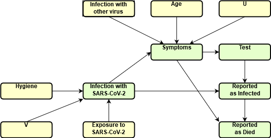
DAG of the process generating data on infected and deceased individuals due to SARS-CoV-2

While the causal graph might be a reasonable description for the reporting mechanism across countries and over time, the details of the causal relationships certainly were neither time-constant nor identical across coutries. Below we describe the situation as it likely existed in March of 2020 in Germany as an example:

For an individual to be reported to be infected with SARS-CoV-2, there are two main causal influneces: whether the person is in fact infected with that virus and whether a PCR test was performed. If we assume that the PCR test used is perfect (i.e. has no type I error nor a type II error), we can model this relationship deterministically as $ReportedInfection := f(Test, Infection)$. Note that the assumption of a perfect test also allows us to disregard any causal influence from $OtherInfection$ to $ReportedInfection$, which would be the case if the test accidently would show positive outcomes in cases where the person does not have SARS-CoV-2, but a similar infection (e.g. other corona viruses), a problem of early antibody tests.
In Germany, an individual is tested for SARS-CoV-2 if they are symptomatic and/or have had recent contact with a person known to be SARS-CoV-2-positive. Again, for simplicity, we assume that this is a strict rule-based (and stable) mechanism.⁷ The structural assigment is $Test := g(Symptoms, ContactInfected)$.

A person’s symptoms are determined by them being infected by the SARS-Cov-2 virus, other viruses causing respiratory diseases, age, pre-existing conditions, as well as other unspecified and unobserved factors (e.g. genetics). The assignment is \[\begin{equation} Symptoms := h(Infection, InfectionOther, Age, PreCondition, U) \end{equation}\] and the assignment is probabilistic due to $U$ being treated as a noise term. As we define symptoms to include the value “death”, this mechanisms has to fully explain a person’s likelihood to die with and without the virus.
The infection mechanism is modelled as a probablistic function of personal hygiene and exposure to the virus: \[\begin{equation} Infection := h(Hygiene, Exposure, V) \end{equation}\]
finally, a person is reported to have died of SARS-CoV-2 if the person has been positively tested for the virus and has died (one of the possible values of the symptom): \[\begin{equation} ReportedDeath := h(ReportedInfection, Symptoms) \end{equation}\] We assume this to be a simple and deterministic mechanism.

4.5.1.1 Reasoning about interventions and counterfactuals

The model now allows us to reason about certain interventions that affect the reported numbers of infected and deceased.

4.5.1.1.1 No virus

The most important one is certainly the counterfactual question of what would happen if there were no SARS-CoV-2 virus out there, which serves as a baseline model that allows us to compare the pandemic situation to a “normal” one. Technically, this amounts to replacing the assignment for variable $Infection$ to \[\begin{equation} Infection := 0 \end{equation}\] As this is just a hypothetical intervention, let us assume that it is atomic, i.e. we assume that the rest of the model is not changed by this intervention. Most importantly, the assignment $Symptoms := h(Infection, InfectionOther, Age, PreCondition, U)$ is still in place, it’s just that the value of one of the inputs is $0$ in the entire population. As $Symptoms$ was defined to be a categorical variable including the value “death”, we can use the model to compare two distributions in the population, one with and one without the virus. The difference tells us the additional deaths due to SARS-CoV-2 virus rather than just the numer of deaths associated with SARS-CoV-2 (which is what $ReportedDeath$ is capturing). This information is important because we ultimately want to understand how deadly the disease acutally is, i.e. how many deaths it causes, not just how prevalent it is in people how are dying. With the median age of reported deaths with the virus being at around 80 and the probability of a person at 80 to die within 12 months being at around 5%, this is non-negligible.

4.5.1.1.2 Changing testing strategy

expanding test capacities comparing numbers across countries with (very) different test strategies random testing

4.5.2 Evolving Symptoms

To model the evolution of symptoms over time, we need to switch from a time series summary graph to a full time graph.

Typically you will find a notation similar to $P(Y|X) = f(X)$ where $X$ is called a feature set or a vector/matrix of features. I use the term information set to deliberately distinguish between the notion of all the information you have available for a customer. The information set is abstract and represents information in potentially very different formats, e.g. order data in your data base, the recorded call with the customer service team, or the customer’s product reviews. Feature engineering is the step where this information is transformed into a format that can be used by ML algorithms: the order data could be transformed into multiple features, e.g. the total revenue in past 30 days, total revenue in past 180 days, the number of days the customer put an order in; the recorded call can transformed into days since the latest customer service contanct, length of the call, length of waiting in line and whether or not the issue was resolved; the product reviews are transformed into word embeddings.↩︎
Early numbers suggested that, after accounting for asymptomatic and untested cases, the SARS-CoV-2 virus might be similarly fatal as the influenza. This conclusion often neglected the fact that influenza-patients usually get the full treatment, but that faster spreading of SARS-CoV-2 might concentrate severe cases to a shorter time period, overwhelming the capaicities for treatment and therefore increasing the CFR.↩︎
In reality, this assumption was violated. Over the course of the epidemic, testing capabilities have increased in most countries and tests have been expanded over time. In some countries and regions, asymptomatic persons have been tested as well, even if there was no known contact with another infected person. We discuss this in more detail when we take a look at the full time graph of the model.↩︎

	\(Y^{\Gamma;do(X:=0)} = 0\)	\(Y^{\Gamma;do(X:=0)} = 1\)
\(Y^{\Gamma;do(X:=1)} = 0\)	“Lost Cause”	“Do-Not-Disturb”
\(Y^{\Gamma;do(X:=1)} = 1\)	“Persuadable”	“Sure Things”